How Is Marginal Cost Found

Cost added by producing i additional unit of a product or service

In economics, the marginal cost is the change in the total cost that arises when the quantity produced is incremented, the price of producing additional quantity.^[one] In some contexts, it refers to an increment of ane unit of output, and in others it refers to the rate of change of total toll as output is increased by an infinitesimal amount. As Effigy i shows, the marginal cost is measured in dollars per unit of measurement, whereas full toll is in dollars, and the marginal price is the gradient of the total cost, the charge per unit at which it increases with output. Marginal price is different from average cost, which is the total cost divided by the number of units produced.

At each level of production and time period being considered, marginal cost includes all costs that vary with the level of product, whereas costs that do non vary with production are fixed. For example, the marginal cost of producing an machine will include the costs of labor and parts needed for the additional auto but not the fixed cost of the factory building that do not change with output. The marginal toll can be either short-run or long-run marginal toll, depending on what costs vary with output, since in the long run even edifice size is chosen to fit the desired output.

If the cost function $C$ is continuous and differentiable, the marginal cost $MC$ is the beginning derivative of the cost function with respect to the output quantity $Q$ :^[two]

MC(Q)={\frac {\ dC}{\ dQ}}.

If the cost function is not differentiable, the marginal toll tin can be expressed as follows:

MC={\frac {\Delta C}{\Delta Q}},

where $\Delta$ denotes an incremental change of one unit of measurement.

Short run marginal cost [edit]

Short run marginal toll is the alter in total cost when an additional output is produced in the short run and some costs are fixed. On the right side of the page, the short-run marginal cost forms a U-shape, with quantity on the ten-axis and cost per unit on the y-axis.

On the short run, the business firm has some costs that are fixed independently of the quantity of output (e.g. buildings, machinery). Other costs such equally labor and materials vary with output, and thus prove up in marginal cost. The marginal cost may beginning decline, every bit in the diagram, if the additional cost per unit is high if the business firm operates at as well low a level of output, or it may start flat or rise immediately. At some bespeak, the marginal price rises every bit increases in the variable inputs such as labor put increasing pressure on the fixed assets such every bit the size of the building. In the long run, the house would increase its fixed assets to correspond to the desired output; the short run is defined equally the catamenia in which those assets cannot exist changed.

Long run marginal cost [edit]

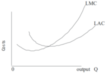
The long run is defined as the length of time in which no input is fixed. Everything, including edifice size and mechanism, tin can exist chosen optimally for the quantity of output that is desired. As a upshot, even if brusk-run marginal toll rises because of chapters constraints, long-run marginal cost can be abiding. Or, there may be increasing or decreasing returns to calibration if technological or management productivity changes with the quantity. Or, at that place may exist both, as in the diagram at the correct, in which the marginal toll offset falls (increasing returns to scale) and then rises (decreasing returns to scale).^[3]

Cost functions and relationship to average cost [edit]

In the simplest example, the total cost function and its derivative are expressed as follows, where Q represents the production quantity, VC represents variable costs, FC represents fixed costs and TC represents total costs.

Fixed costs represent the costs that do not modify as the production quantity changes. Fixed costs are costs incurred by things like rent, building space, machines, etc. Variable costs modify as the product quantity changes, and are often associated with labor or materials. The derivative of fixed cost is zilch, and this term drops out of the marginal cost equation: that is, marginal toll does not depend on stock-still costs. This can be compared with boilerplate full toll (ATC), which is the total cost (including fixed costs, denoted C₀) divided by the number of units produced:

ATC={\frac {C_{0}+\Delta C}{Q}}.

For discrete calculation without calculus, marginal toll equals the change in full (or variable) price that comes with each boosted unit of measurement produced. Since fixed cost does not change in the short run, it has no outcome on marginal cost.

For case, suppose the total toll of making 1 shoe is $30 and the total price of making 2 shoes is $forty. The marginal cost of producing shoes decreases from $30 to $ten with the production of the second shoe ($xl – $30 = $10).

Marginal cost is non the cost of producing the "next" or "last" unit.^[4] The cost of the last unit is the same as the cost of the first unit of measurement and every other unit. In the short run, increasing product requires using more of the variable input — conventionally assumed to be labor. Adding more labor to a fixed capital stock reduces the marginal production of labor because of the diminishing marginal returns. This reduction in productivity is not express to the additional labor needed to produce the marginal unit of measurement – the productivity of every unit of measurement of labor is reduced. Thus the toll of producing the marginal unit of output has two components: the cost associated with producing the marginal unit and the increase in average costs for all units produced due to the "harm" to the entire productive process. The showtime component is the per-unit of measurement or average cost. The 2d component is the modest increase in cost due to the police force of diminishing marginal returns which increases the costs of all units sold.

Marginal costs can also be expressed equally the cost per unit of labor divided past the marginal production of labor.^[5] Denoting variable price every bit VC, the constant wage rate as westward, and labor usage as 50, we have

MC={\frac {\Delta VC}{\Delta Q}}

\Delta VC={w\Delta 50}

MC={\frac {w\Delta Fifty}{\Delta Q}}={\frac {w}{MPL}}.

Here MPL is the ratio of increment in the quantity produced per unit increment in labour: i.e. ΔQ/ΔL, the marginal product of labor. The last equality holds because ${\frac {\Delta L}{\Delta Q}}$ is the change in quantity of labor that brings about a i-unit change in output.^[6] Since the wage rate is assumed constant, marginal cost and marginal product of labor have an changed relationship—if the marginal product of labor is decreasing (or, increasing), then marginal price is increasing (decreasing), and AVC = VC/Q=wL/Q = due west/(Q/L) = w/AP₅₀

Empirical data on marginal cost [edit]

While neoclassical models broadly assume that marginal cost will increase equally production increases, several empirical studies conducted throughout the 20th century accept concluded that the marginal price is either constant or falling for the vast majority of firms.^[7] Virtually recently, former Federal Reserve Vice-Chair Alan Blinder and colleagues conducted a survey of 200 executives of corporations with sales exceeding $x million, in which they were asked, among other questions, about the structure of their marginal price curves. Strikingly, just 11% of respondents answered that their marginal costs increased as production increased, while 48% answered that they were constant, and 41% answered that they were decreasing.^[viii] ^: 106 Summing upwardly the results, they wrote:

...many more than companies land that they accept falling, rather than rising, marginal price curves. While there are reasons to wonder whether respondents interpreted these questions about costs correctly, their answers pigment an prototype of the cost structure of the typical firm that is very different from the ane immortalized in textbooks.

— Asking About Prices: A New Approach to Understanding Price Stickiness, p. 105^[8]

Many Post-Keynesian economists have pointed to these results as evidence in favor of their ain heterodox theories of the firm, which generally assume that marginal toll is constant as product increases.^[seven]

Economies of calibration [edit]

Economies of calibration employ to the long run, a span of time in which all inputs tin exist varied by the business firm so that there are no fixed inputs or stock-still costs. Production may be subject to economies of scale (or diseconomies of scale). Economies of scale are said to exist if an additional unit of output tin can be produced for less than the average of all previous units – that is, if long-run marginal cost is below long-run average cost, and then the latter is falling. Conversely, in that location may be levels of production where marginal price is higher than average toll, and the boilerplate cost is an increasing part of output. Where there are economies of scale, prices set at marginal cost will fail to cover full costs, thus requiring a subsidy.^[9] For this generic case, minimum boilerplate price occurs at the bespeak where average cost and marginal cost are equal (when plotted, the marginal cost curve intersects the boilerplate cost curve from below).

Perfectly competitive supply curve [edit]

The portion of the marginal cost curve above its intersection with the average variable cost curve is the supply curve for a firm operating in a perfectly competitive market (the portion of the MC curve below its intersection with the AVC curve is non part of the supply curve because a firm would not operate at a toll below the shutdown indicate). This is not true for firms operating in other marketplace structures. For example, while a monopoly has an MC bend, information technology does non have a supply curve. In a perfectly competitive market, a supply curve shows the quantity a seller is willing and able to supply at each price – for each price, at that place is a unique quantity that would be supplied.

Decisions taken based on marginal costs [edit]

In perfectly competitive markets, firms decide the quantity to exist produced based on marginal costs and sale toll. If the sale price is higher than the marginal cost, then they produce the unit and supply it. If the marginal price is college than the price, it would not be profitable to produce it. And so the production volition be carried out until the marginal cost is equal to the sale price.^[10]

Human relationship to fixed costs [edit]

Marginal costs are not affected by the level of fixed cost. Marginal costs can be expressed as ∆C/∆Q. Since fixed costs do not vary with (depend on) changes in quantity, MC is ∆VC/∆Q. Thus if fixed cost were to double, the marginal cost MC would non exist affected, and consequently, the profit-maximizing quantity and price would not change. This can exist illustrated by graphing the short run total cost curve and the short-run variable cost curve. The shapes of the curves are identical. Each bend initially increases at a decreasing rate, reaches an inflection betoken, then increases at an increasing rate. The only divergence between the curves is that the SRVC curve begins from the origin while the SRTC curve originates on the positive function of the vertical axis. The distance of the beginning point of the SRTC above the origin represents the fixed toll – the vertical distance between the curves. This distance remains constant as the quantity produced, Q, increases. MC is the slope of the SRVC curve. A change in fixed cost would exist reflected by a change in the vertical distance between the SRTC and SRVC curve. Any such change would take no result on the shape of the SRVC curve and therefore its gradient MC at any betoken. The changing law of marginal cost is similar to the changing law of boilerplate price. They are both subtract at starting time with the increase of output, then get-go to increase after reaching a certain scale. While the output when marginal cost reaches its minimum is smaller than the boilerplate total toll and average variable cost. When the average total cost and the boilerplate variable cost attain their lowest point, the marginal cost is equal to the average cost.

[edit]

Of great importance in the theory of marginal cost is the distinction between the marginal individual and social costs. The marginal private price shows the cost borne by the firm in question. It is the marginal individual cost that is used by business organization decision makers in their turn a profit maximization behavior. Marginal social cost is similar to private cost in that information technology includes the cost of private enterprise but too any other toll (or offsetting benefit) to parties having no directly association with purchase or sale of the product. It incorporates all negative and positive externalities, of both production and consumption. Examples include a social toll from air pollution affecting tertiary parties and a social benefit from influenza shots protecting others from infection.

Externalities are costs (or benefits) that are not borne by the parties to the economic transaction. A producer may, for instance, pollute the environs, and others may bear those costs. A consumer may eat a good which produces benefits for society, such every bit instruction; because the individual does not receive all of the benefits, he may eat less than efficiency would suggest. Alternatively, an individual may be a smoker or alcoholic and impose costs on others. In these cases, product or consumption of the skillful in question may differ from the optimum level.

Negative externalities of production [edit]

Negative Externalities of Production

Much of the time, private and social costs do not diverge from i another, but at times social costs may be either greater or less than private costs. When the marginal social cost of production is greater than that of the private cost function, in that location is a negative externality of product. Productive processes that event in pollution or other environmental waste are textbook examples of production that creates negative externalities.

Such externalities are a result of firms externalizing their costs onto a third party in order to reduce their own full cost. Equally a result of externalizing such costs, we meet that members of society who are not included in the business firm will exist negatively affected by such behavior of the house. In this case, an increased cost of production in social club creates a social cost bend that depicts a greater toll than the individual cost curve.

In an equilibrium state, markets creating negative externalities of production will overproduce that practiced. As a issue, the socially optimal production level would be lower than that observed.

Positive externalities of product [edit]

Positive Externalities of Production

When the marginal social cost of product is less than that of the private toll function, at that place is a positive externality of production. Production of public goods is a textbook instance of production that creates positive externalities. An instance of such a public good, which creates a departure in social and private costs, is the production of didactics. It is often seen that education is a positive for whatever whole guild, likewise as a positive for those directly involved in the market place.

Such production creates a social cost curve that is beneath the individual cost curve. In an equilibrium state, markets creating positive externalities of product will underproduce their good. As a result, the socially optimal product level would be greater than that observed.

Relationship between marginal price and average total cost [edit]

The marginal cost intersects with the average total cost and the average variable cost at their everyman bespeak. Accept the [Relationship between marginal toll and average total price] graph as a representation.

Relationship between marginal cost and average total price

Say the starting point of level of output produced is northward. Marginal cost is the change of the total cost from an additional output [(n+1)th unit]. Therefore, (refer to "Average cost" labelled picture on the right side of the screen.

In this case, when the marginal cost of the (n+1)thursday unit is less than the boilerplate cost(north), the average cost (n+one) will get a smaller value than boilerplate cost(north). Information technology goes the contrary manner when the marginal cost of (north+1)th is higher than average cost(n). In this example, The average price(north+1) will be higher than boilerplate cost(northward). If the marginal toll is found lying under the average cost curve, it volition curve the average cost curve downwards and if the marginal cost is above the average cost curve, it will bend the average toll curve upwardly. You tin see the table higher up where before the marginal cost bend and the boilerplate cost curve intersect, the average price curve is downwards sloping, all the same later on the intersection, the average cost bend is sloping upwards. The U-shape graph reflects the law of diminishing returns. A firm can merely produce so much but after the production of (n+i)th output reaches a minimum cost, the output produced after volition only increase the average total cost (Nwokoye, Ebele & Ilechukwu, Nneamaka, 2018).

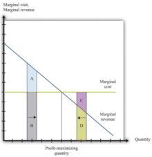
Profit maximization [edit]

The profit maximizing graph on the correct side of the page represents optimal production quantity when both The marginal price and the marginal profit line intercepts. The Black line represents the intersection where the profits are the greatest ( Marginal revenue = marginal toll). The left side of the blackness vertical line marked as "profit-maximising quantity" is where the marginal revenue is larger than marginal price. If a firm sets its production on the left side of the graph and decides to increase the output, the additional revenue per output obtained will exceed the additional cost per output. From the "profit maximizing graph", nosotros could observe that the acquirement covers both bar A and B, meanwhile the cost only covers B. Of course A+B earns you lot a profit only the increment in output to the point of MR=MC yields extra profit that can encompass the revenue for the missing A. The business firm is recommended to increase output to reach (Theory and Applications of Microeconomics, 2012).

On the other paw, the right side of the black line (Marginal revenue = marginal cost), shows that marginal cost is more than marginal revenue. Suppose a firm sets its output on this side, if it reduces the output, the cost will decrease from C and D which exceeds the decrease in revenue which is D. Therefore, decreasing output until the point of (marginal acquirement=marginal price) volition atomic number 82 to an increment in profit (Theory and Applications of Microeconomics, 2012).

References [edit]

^ O'Sullivan, Arthur; Sheffrin, Steven M. (2003). Economic science: Principles in Action . Upper Saddle River, NJ: Pearson Prentice Hall. p. 111. ISBN0-13-063085-3.
^ Simon, Carl; Blume, Lawrence (1994). Mathematics for Economists. W. W. Norton & Visitor. ISBN0393957330.
^ The classic reference is Jakob Viner, "Cost Curves and Supply Curve," Zeitschrift fur Nationalokonomie, 3:23-46 (1932).
^ Silberberg & Suen, The Structure of Economic science, A Mathematical Analysis 3rd ed. (McGraw-Colina 2001) at 181.
^ See http://ocw.mit.edu/courses/economic science/14-01-principles-of-microeconomics-fall-2007/lecture-notes/14_01_lec13.pdf.
^ Chia-Hui Chen, course materials for xiv.01 Principles of Microeconomics, Fall 2007. MIT OpenCourseWare (http://ocw.mit.edu), Massachusetts Institute of Technology. Downloaded on [12 Sept 2009].
^ ^a ^b Lavoie, Marc (2014). Post-Keynesian Economics: New Foundations. Northampton, MA: Edward Elgar Publishing, Inc. p. 151. ISBN978-1-84720-483-vii.
^ ^a ^b Blinder, Alan South.; Canetti, Elie R. D.; Lebow, David E.; Rudd, Jeremy B. (1998). Asking Nigh Prices: A New Approach to Understanding Toll Stickiness. New York: Russell Sage Foundation. ISBN0-87154-121-one.
^ Vickrey W. (2008) "Marginal and Average Price Pricing". In: Palgrave Macmillan (eds) The New Palgrave Lexicon of Economics. Palgrave Macmillan, London^{[ ISBN missing ]}
^ "Piana V. (2011), Refusal to sell – a key concept in Economics and Management, Economics Web Constitute."

External links [edit]

Bio, Full (2021-05-19). "Marginal Cost Of Production Definition". Investopedia . Retrieved 2021-05-28 .
Nwokoye, Ebele Stella; Ilechukwu, Nneamaka (2018-08-06). "Affiliate FIVE THEORY OF COSTS". ResearchGate . Retrieved 2021-05-28 .
"Theory and Applications of Microeconomics - Table of Contents". 2012 Book Archive. 2012-12-29. Retrieved 2021-05-28 .